Yonatan Zunger’s Blog

Last time, we walked through some of the history of quantum mechanics and came out with the Schrödinger Equation, the master equation of nonrelativistic quantum mechanics. Much of what we’ll do in this course will involve solving this equation in a variety of interesting cases; but before we begin, it’s worth plunging a bit more deeply into the equation itself and seeing what we can learn just from its structure. Among other things, we’ll see the relationship of the abstract vectors we get from the linear algebra approach to the functions we use in the differential-equation approach; see the (rather simple) way that real systems evolve over time; and encounter the fundamental limitations on measurement in quantum mechanics.

The relationship between vectors and functions

We wrote down the Schrödinger equation in terms of differential operators acting on functions:

.

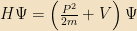
Here Ψ is a complex-valued wave function, and its magnitude squared can be interpreted as a probability — specifically, for any linear operator A built up out of X’s and P’s and so on,

.

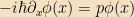
We also identified some important operators:

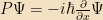
We didn’t write down the first equation last time, but it’s somewhat obvious, and I’m writing it for completeness; the X operator simply means “multiply by x.”

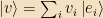
Let’s apply some of our linear algebra to these equations. Ψ is acting like a vector in the space of functions, so let’s explicitly denote it as a vector and write it as . How does this abstract vector relate to the function ? It’s the same as the relationship of an abstract vector in an abstract vector space to the explicit column of numbers as which we normally write it. Those numbers are simply the coefficients in , where the are the basis vectors of the space. Similarly, the are the coefficients of in a basis expansion — specifically, the basis of eigenvectors of X.

To see the details, let’s look more carefully at the eigenvectors of X. If we think about these as functions, then they must satisfy . Now, the only way that xφ(x) can be proportional to φ(x) is if φ vanishes at all but (at most) a single value of x. The function which satisfies this is the Dirac delta function:

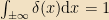
This function is an infinitely high spike centered at the origin.¹ It satisfies the useful relationship

,

which follows directly from the definition; it’s the continuous analogue of the Kronecker delta . The eigenfunctions of X are simply Dirac deltas centered at every possible value of x:

.

These obviously form a basis for the set of functions on the real line. In fact, it’s not hard to expand any function in terms of them:

.

i.e., the function values are exactly the coefficients of f in the X-basis.

Why did I bother with this? Well, because we can easily consider other bases, too. For example, the eigenfunctions of P satisfy

;

i.e.,

.

The subscript “p” simply indicates which eigenfunction we’re looking at.2 The fact that I’ve written these as functions is simply the expansion of the P eigenvectors in terms of the X eigenvectors:

.

So if I’m talking about some arbitrary state vector , (I’ll refer to the wave function as a “state vector” often, especially when emphasizing the fact that it’s a vector in this abstract Hilbert space) I can expand it in the X-representation, i.e. as a function of x, or in the P-representation, i.e. as a function of p, and it’s the same vector. The two are related by a simple change of basis:

.

In the first step, I used the fact that extracts the component of parallel to , i.e. . In the second step, I used the fact that the x’s form a basis, so . This operation is an extremely common move in QM, and is generally referred to as “inserting a complete set of states.” In the third step, I used the expansion of the in terms of the ‘s, above. Thus the function of position and the function of momentum are related by a simple Fourier transform! In general, we will be able to switch between arbitrary pairs of basis functions by the same method. While most of the resulting integrals won’t be quite as simple as Fourier transforms, they will be reasonably manageable. We will also show later on that, whenever q and p are canonically conjugate coordinates, they will have the same relationship as x and p and thus really will have a Fourier transform relationship.

Now let’s look at our expression for expectation values. Rewritten in vector language, it says

.

(The expression of this as an integral simply follows from inserting two complete sets of x-states, on either side of the A. Exercise: Show this in detail)

Note, also, that using this probability interpretation there is a very clear interpretation of the meaning of being an eigenvector of A; if , then . (Where we used the normalization relationship, ; note how in vector notation, this is just a statement that is a unit vector) An eigenstate of an operator is simply a state in which we have a definite value of the operator — i.e., a spike probability distribution.

We’ll routinely move back and forth between the function (differential-equation) description and the algebra (state-vector) description, depending on which is more convenient.

The Uncertainty Principle

Now let’s the fact that operators — or at least, Hermitian operators, which have real eigenvalues — seem to correspond to physically observable quantities with our earlier demonstration that commuting operators share eigenvectors. This means that if two operators A and B commute, then can simultaneously be an eigenstate of both operators — i.e., it can be described as having definite values of both quantities at once. So if we have a collection of physical observables in a system, it is natural to try to build a maximal set of commuting observables, and pick as our basis their simultaneous eigenstates. For reasons we’ll see later, we’ll almost always want the Hamiltonian to be one of these operators, even if it greatly restricts our choices of other operators to add to the set.

What happens if they don’t commute? Let’s assume that , and that we are in some fixed state . Let us define the operator

.

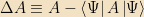
The second term is simply a number; this operator measures the deviation of a measurement of A from the mean. The expectation value of its square is the variation, a.k.a. the mean-square deviation:

.

The square root of this term is simply the standard deviation of measurements of A from the mean. (Note that, if , then , and so ; an eigenstate of A has a definite value of A, and so its statistical dispersal is zero) It turns out that we can prove a fascinating inequality, for any operators A and B and any state :

This is the Heisenberg uncertainty principle.³ Before we analyze it, let’s prove it. First, we prove the Cauchy-Schwarz inequality:

.

Exercise: Show this. Hint: Start from the fact that the norm of must be ≥0, for any λ.

If we let , and , this then means that

.

Now note that

.

(The latter quantity is called the anticommutator; these show up a lot in relativistic QM) Now, the commutator of two Hermitian operators is anti-Hermitian:

and similarly, the anticommutator of two Hermitian operators is Hermitian. It’s trivial to see that the eigenvalues of any Hermitian operator must be real, and of an anti-Hermitian operator must be imaginary; simply write the operators in the basis where they are diagonal. That in turn implies that the expectation value of an (anti-)Hermitian operator must be real (imaginary), since we can expand in terms of the basis vectors which diagonalize the operator, and then write out the sum. And since we’ve now written as a sum of a purely real and a purely imaginary term, it follows that . Since both of the quantities on the right are nonnegative, the theorem immediately follows. ♦

So now that we’ve proven the uncertainty principle, what does it mean? It means that, if two operators don’t commute, then no state can be in a simultaneous eigenket of both, or have a definite value of both; in fact, the product of the errors in measuring both of the quantities is bounded from below.

Let’s be concrete;  take the operators X and P. Their commutator is easy to work out: for any ,

,

and thus . Then for any physical state, no matter what it is, no matter what the Hamiltonian or potential function or quality of the experiment,

.

You can physically visualize why this happens in terms of the explicit eigenfunctions we worked out earlier for X and P. If you are in an X-eigenstate, i.e. , then you are by no means in a P eigenstate; in fact, you are in a linear combination of infinitely many P eigenstates with different values of momenta, the coefficients coming from a Fourier transform. It should hardly be surprising, then, that measuring P in such a circumstance will lead to an infinite range of possible values. Here , and so . Likewise, if we were in a P-eigenstate, we would be in an infinite superposition of X-eigenstates. Other functions sit between these two extremes.

Exercise: Let 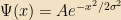be a normalized Gaussian. Find A so that . Evaluate , , , and . (The integrals are all standard; you should be able to do them by hand) Show that for any σ.

This form of Ψ is often referred to as a wave packet. It saturates the position-momentum uncertainty relationship, and is reasonably localized in space. (With the definition of “reasonably” being “within σ”) As such, it’s a very “particle-like” state for a system to be in.⁴

The uncertainty principle took many years for people to fully digest, and physicists spent a great deal of time⁵ trying to build thought experiments (and physical experiments) designed to defeat it, simultaneously measuring the position and momentum of a particle. In every case it failed; generally, the failure takes the form of the physical action required to measure one of the quantities disturbing the other quantity by a certain minimum amount. To take a simple example, consider Heisenberg’s original motivating example, using a microscope to measure the position and velocity of a particle. In order to see the particle, we must bounce a photon off of it. But the ability to resolve the particle’s position is bounded below by the wavelength, so we need ; but this implies that the photon imparts its own energy to the particle, and its own momentum: . So . There are obviously many possible refinements of this idea; see the Wikipedia article for a good place to start exploring if you’re interested.

The Time-Independent Equation

Very often, the Hamiltonian has no explicit time dependence. In this case, it’s possible to separate the Schrödinger equation into two simpler equations. From a differential equation perspective, we can separate the variables by conjecturing that we can write . Then the Schrödinger equation becomes:

Dividing both sides (on the left, if you want to be careful) by gives

.

The left-hand side of this equation is a function only of x; the right-hand side, only of t. The only way these two functions can therefore be equal to one another is if they’re both equal to a constant, which we’ll denote by E. (This will be our one exception to the constants-are-lowercase rule) The right-hand side is now simple to solve:

.

The left-hand side is

.

This is the time-independent Schrödinger equation, and is generally much easier to solve than the time-dependent version. We can immediately see that it is simply an eigenvalue equation for H; and knowing that H is our Hamiltonian, we can immediately interpret the physical meaning of E as the energy of the state.

Time Evolution

If we write down the Schrödinger equation for a time-independent Hamiltonian in vector notation,

we can solve it in a very formal sense:

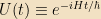
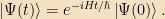
The exponential of an operator is simply defined by its Taylor series; if you write out the infinite sum, it’s obvious that this solves the differential equation. The operator on the right-hand side is known as the time-evolution operator, , since it transforms kets at time T to the corresponding kets at time T+t.⁶ This equation is most useful if we recall that the eigenvectors of H form a basis, and expand our initial condition in those terms;

,

where n is some index that runs over the eigenvectors of H. Then

This is how kets evolve over time. Note that if is an eigenket of H, then there is only one term in this sum, and the “time-evolution” of is nothing more than a phase changing over time; since all of our physically measurable quantities take the form , this means that the expectation value of any operator that doesn’t have an explicit time-dependence built in is going to be constant over time. Overall phases in the wave function have no physical meaning! (Which if you recall, is exactly why we picked complex numbers for our wave function in the first place)

If on the other hand is not an eigenket of H, there are multiple terms in the sum, and their relative phases will change over time; this means that expectation values can evolve nontrivially. We’ll see several examples of this shortly.

Note one other thing: For any observable A, . Apart from the interesting fact that time-evolution just looks like a change of basis, you should note that if , then (by the Taylor series), and so the U’s cancel out; the expectation value of A is a constant! The converse is, true, too; if for any initial condition, then A must commute with H.

Proof: By Taylor expansion,

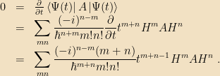
For this to vanish for every t, the coefficient of each power of t must vanish independently; but the coefficient of is simply . ♦

Thus an operator corresponds to a conserved quantity if and only if it commutes with the Hamiltonian. This means that sets of commuting observables which include the Hamiltonian are particularly interesting; they represent sets of simultaneously measurable conserved quantities. Maximal sets of commuting observables are even more interesting; if two eigenkets of such a set have the same eigenvalues under each operator, then (by definition) there is no other quantity which we could measure which would distinguish the two; the two kets must correspond to the same physical state. We can therefore label the eigenkets of such a CSCO by their eigenvalues under each of the operators, and those labels form a complete description of the state of the system in each eigenket. This relatively simple statement will turn out to have profound implications later — in quantum mechanics, when two particles are identical, they’re really identical.

Next Time: A concrete example: The two-state system and nuclear magnetic resonance.

---

¹ Dirac proposed this “function” for exactly this purpose, and mathematicians proceeded to spend decades arguing over whether or not it was a bona fide function. This required some careful rethinking of the definition of functions, some work in measure theory, and so on, and the practical upshot was that yes, this whole thing works just fine. Physicists pretty much ignored the entire controversy.

2 Note that these eigenfunctions aren’t normalized; is in fact infinite when . This is actually an annoying corner case in many of our discussions; the proper way to handle this is to assume that space has a finite extent L, normalize the functions there, and take the limit at the end. It’s not actually especially illuminating to do this, so for the rest of this course, unless explicitly indicating otherwise, I will leave planewaves unnormalized, and simply take it as implicit that whenever computing expectation values etc. with them, one should do this normalization.

3 Heisenberg considered this his most important discovery; the equation — specialized to the case of x and p — is carved on his tombstone.

⁴ The entire discussion over “particle-wave duality” was an artifact of the confusion in the early 20th century, especially in the aftermath of de Broglie’s paper, when the two concepts were considered to have very distinct physical meanings. From a modern perspective, the distinction is purely semantic. A system is in a “particle-like” state when it has a fairly definite value of position, i. e. is small; it is in a “wave-like” state when it has a fairly definite value of momentum (as a free plane wave does), i.e. is small. But these two states are simply endpoints of a continuum; there is nothing particularly privileged about one or the other.

⁵ Bohr and Einstein famously spent extraordinary amounts of time, especially at the Copenhagen conference in 1925, debating these; every day, Einstein would come up with a (generally extremely subtle) objection to the quantum results, and Bohr would (after much hand-wringing) come back with an explanation. Reading up on their debates is fascinating.

⁶ Note that we can still define in the case where H does have an explicit time-dependence, but the formula for it isn’t as simple; it’s the solution to the differential equation.