Yonatan Zunger’s Blog

And now for the first contentful post about quantum mechanics. It’s wild, wonderful, exciting… okay, not really. It’s the mathematical prelude, an overview of some key physical constants and some key bits of linear algebra which we’ll use rather extensively going forwards. This isn’t meant to be deep, or to be an introduction to linear algebra; it’s a way to establish the notations we’ll be using, and to point out the facts which will happen to be important to us later on.

Some useful numbers

The fundamental physical constant associated with Quantum Mechanics is Planck’s constant, . Planck also defined a “reduced” constant, ,¹ and it quickly became clear that this constant was the one which actually showed up in equations; so nowadays when anyone refers to Planck’s constant they’re referring to this. (On the rare occasions when the original number is needed, one simply uses instead)

Our unit of length will be the Angstrom, , and our unit of energy will be the electron-volt, the energy that an electron acquires when moving through a potential difference of one volt, . These are convenient for what we will need — a typical atom is 1-3Å across, binding energies in atoms are on the order of a few eV, and so on. A few combinations which are particularly useful to remember are:

Atomic binding energies are generally on the order of a few eV; the weak hydrogen-hydrogen bonds used in biological systems are a few meV; nuclear binding energies are a few MeV. The largest particle accelerators have beam energies on the order of tens of TeV per particle; the most energetic cosmic ray ever observed was a proton with an energy of about , about the same as a baseball going at 60mph.

A bit of linear algebra

Bibliographic note: My favorite more detailed text on this subject is chapter 1 of Sakurai. If you’re of a somewhat mathematical bent, that book is a great place to start.

And now for a lightning review of linear algebra. This is not meant to teach you linear algebra; if you tried to learn it from this, your head would probably explode. It’s just a way for me to review the key points, describe the rather oddball notation that we use in quantum mechanics, and point out a few key facts which we’ll use over and over later on. The hope is that you’ll read over this and say “yeah, yeah, obvious… incomprehensible, but obvious… blah blah… ok.” If you don’t say that, then stop me and ask, because this part needs to be clear. (Also, if you need a linear algebra refresher, the  Wikipedia articles are an OK place to start)

Vector spaces, kets: A vector space is any collection of objects which can be added and multiplied by numbers. (aka, scalars) In quantum mechanics, we will generally be concerned with complex vector spaces, i.e. ones where these constants are complex numbers. Some common examples of vector spaces are the space of vectors in the plane, and the space of functions on the real line. We will denote the vector named “x” by . (This is the notation standard in quantum mechanics; it’s different than the one commonly used in mathematics, but it turns out to be surprisingly useful) Such vectors are commonly called “kets,” (Dirac’s name) and correspond to the column vectors familiar from high school algebra. We will label our kets with an amazing bestiary of things, including Roman letters, Greek letters, and numbers. We’ll use lower-case letters from all alphabets for our scalars.

Inner products, bras, adjoints: All of the vector spaces we will be interested in are inner product spaces — i.e., there is an inner (dot) product which takes two vectors and gives a scalar. But we’re going to be a bit more careful than this standard statement. Instead, we’ll say this: For every vector space, there exists a dual vector space; this is the pairing of column vectors to row vectors. These row vectors are denoted by , and are called “bras.” The standard pairing between rows and columns is called the Hermitian adjoint, the adjoint or (in speech) simply the “dagger:” . This dagger is “anti-linear:”

.

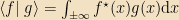
In simpler terms, the dagger is the complex conjugate of the transpose. For complex vector spaces, this dagger will take the place of the ordinary transpose everywhere. We define the inner (dot) product to be a product of a bra and a ket: , which is a number. Note that you can immediately tell if something is a bra, a ket, or a scalar, simply by counting the pointy bits; this is often useful.²

For vectors on a plane, if and (where and are the unit vectors along the axes), then . For functions on the real line, the standard inner product is

.

Note that this doesn’t actually work as an inner product over arbitrary functions, since the integral could diverge; so the interesting inner product space is the space of square-integrable functions, i.e. the set of functions for which this integral is finite. We’ll use this space all the time.

The norm of a vector is the square root of its dot product with itself. The formal definition of an inner product also states that every vector must have nonnegative norm, and only the zero vector has norm zero. See the Wikipedia page for more about inner products if you want details.

In QM you’ll often see the term “Hilbert space” bandied about. Technically, a Hilbert space is an inner product space which is Cauchy-complete; in practice, fewer than one physicist in fifty could probably tell you that definition from memory, because it’s of very little practical use in QM. However, it does turn out that all of the vector spaces we’ll be interested really are Hilbert spaces, and so they are commonly referred to as such and are often denoted by  . Physicists will also sometimes abuse this notation even more and use the term “Hilbert space” only for infinite-dimensional Hilbert spaces, like spaces of functions, and “vector space” for finite-dimensional ones; there is no particularly good reason for this.

Operators: A linear operator (or just “operator” for short) on a vector space is something which maps vectors onto other vectors, which is linear. (i.e., a matrix, but for general vector spaces they’re typically called operators) We’ll denote operators by capital Roman letters, so is a vector. Operator multiplication isn’t commutative; order matters. The commutator of two operators is defined to be

.

Note that if you multiply a ket and a bra in the “wrong order,” you get an operator; you can tell that from the fact that when you multiply it by a ket on the right, you get a ket back.

Operators can be acted on with daggers, too: that dagger is defined by 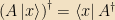for every vector . In practice, the adjoint of an operator is the complex conjugate of its transpose, just like with vectors. Like transposes, daggers reverse the order of multiplication: . (As follows from the definition of the dagger and the associative law) The “identity matrix” is the operator which maps every vector onto itself, and will commonly simply be denoted as “1.”

Operators on vectors in a plane are simply 2×2 matrices. Operators on the space of functions are linear operators; e.g., derivatives are linear operators. The product of two operators is an operator, so , , etc., are all linear operators.

An operator is called “Hermitian” if , “normal” if , and “unitary” if .

Hermitian 2×2 matrices have the form , where all of the coefficients in the matrix are real numbers. Unitary 2×2 matrices have the form ; i.e., they’re simply rotation matrices.

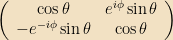
Since we can form polynomials out of operators, we can also form functions of them (or at least, analytic functions of them) by means of Taylor series. One thing that we will do particularly often is exponentiate. A useful fact is that, if , then . (Exercise: Prove it) Also, . Together, these two facts imply that if is Hermitian, then is unitary, for any real number t. In fact, the converse is also true: every unitary operator can be written in the form for some Hermitian A.

Bases: Probably the most important theorem of linear algebra is the Gram-Schmidt theorem, which says that every inner product space has an orthonormal basis. A basis is a set of vectors, which are linearly independent (i.e., no vector in that set can be written as a linear combination of the others) and such that every vector in the entire vector space can be written as a linear combination of those basis vectors; orthonormal means that these basis vectors are orthogonal (the inner product of any two different basis vectors is zero) and normal. (The norm of each basis vector is 1) Each vector space has in fact an enormous variety of bases; but the number of elements in the basis is a constant for any particular vector space, and that number is the dimension of the vector space.

A basis for the set of vectors in the plane is and , the unit vectors in the x and y directions; this vector space is two-dimensional. By Fourier’s Theorem, the set of functions , for every real number k, is a basis for the set of functions on the real line; this vector space is infinite-dimensional.

Given a basis, any vector can be written as its “basis expansion,” i.e. the set of coefficients by which you need to multiply each basis vector in order to get that vector — that’s really what we refer to when we write out a column vector as a column of numbers. Probably the most useful equation you can write about a basis is that, if the form a basis, then

.

(This is easy to see: Write an arbitrary vector as a linear combination of the x’s, multiply this matrix by that vector, and use the fact that )

Bases are by no means unique. In fact, if the set of form an orthonormal basis for a vector space, and is any unitary operator, then the set of are also an orthonormal basis. The example 2×2 unitary matrix above gives you the physical intuition: unitary matrices simply rotate the bases of a space. It is also easy to show that every two orthonormal bases of a vector space are related by this equation; simply let

Then , so this matrix really does relate the two bases; and  .

Thus every unitary operator can be thought of as a change of basis.

If we expand vectors in terms of their basis coefficients, we can also expand operators in the same way. (Which is what we mean when we write out matrices as arrays of numbers) The matrix elements of an operator A are simply . Under a change of basis, ; that way, for every vector, , and so is a vector as well.

Eigen(values, vectors): If is an operator, then is an eigenvector of A, with eigenvalue , if

.

These will turn out to be of tremendous importance in QM. The Spectral Theorem says that, if A is Hermitian, then not only does it have eigenvectors, but the set of its eigenvectors forms a basis of the vector space; i.e., there are as many linearly independent, orthonormal eigenvectors as there are dimensions in the space. This is typically referred to as the “eigenbasis” of A. If the eigenvalues of A are , with respective eigenvalues , then in the eigenbasis A takes on the particularly simple form

If on the other hand we have the eigenvectors of A written in some other basis, then we can form a unitary matrix by simply stuffing the eigenvectors into the columns of a matrix ; that matrix is simply the transformation matrix into the eigenbasis. (So we can write , where D is the diagonal matrix of eigenvalues and P is unitary) Because finding the eigenvectors is equivalent to finding the basis in which A is diagonal, this operation is also referred to as “diagonalization.” The set of eigenvalues is called the spectrum of A. The trace of A is the sum of the eigenvalues; the determinant is their product. (To see this, note that , and that P is unitary) A is positive (semi)definite if all of the eigenvalues are greater than (or equal to) zero; it has an inverse iff none of the eigenvalues are zero. Also, note that since A is Hermitian, the eigenvalues must also be real. (Easy exercise: Show this)³

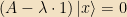
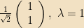
The standard way to find the eigenvalues of a (finite-dimensional) matrix is to note that the eigenvalue equation can be rewritten as ; this equation can only hold for a nonzero vector if the matrix in parentheses is singular, and thus has determinant zero. We therefore take the determinant of the quantity in parentheses and demand that it vanish; for an NxN matrix, this is an N-th order polynomial equation, and the N independent solutions are the eigenvalues. Each individual eigenvalue can then be substituted in to the eigenequation to solve for the corresponding eigenvector.

Example: Let . Then the eigencondition is det . This has solutions . The corresponding eigenvector equations say

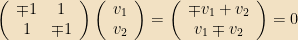
And thus . In order to make these vectors normal, we multiply them each by . (N.B., any multiple of an eigenvector is an eigenvector with the same eigenvalue!) Thus the eigenvectors are

, and

.

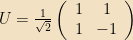
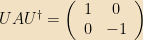
The unitary matrix that moves from the basis in which we originally wrote A into the eigenbasis is simply

; if we apply this change of basis to A,

.

Note that, if two eigenvectors have the same eigenvalues, then any linear combination of those two eigenvectors is also an eigenvector with that eigenvalue. (i.e., the eigenbasis isn’t unique; we can rotate any eigenvector into any other eigenvector and it’s still an eigenbasis)

When we work with an eigenbasis, we will customarily label the basis vectors by their eigenvalues — i.e., .

One of the most important facts about eigenvectors in quantum mechanics is that, if any two Hermitian operators A and B commute, then they have the same set of eigenvectors. (Although they may — will! — have different eigenvalues for each of those vectors. A and B need not even have the same units.)

Proof: Let be the eigenkets of A. First, note that . (Since A is Hermitian) Now, consider the case where A is nondegenerate, i.e. all of its eigenvalues are different. Then , since . Since the eigenvalues are unequal, this must mean that whenever , and so B is diagonal. Now imagine that there are two eigenvectors of A which are degenerate; in that case, there is a corresponding 2×2 submatrix which is not constrained to be diagonal. But this submatrix is Hermitian, because B is, and so it too can be diagonalized. But this diagonalization is just a replacement of those two ‘s with linear combinations of those two; and as we already saw, whenever two eigenvalues are degenerate we can rotate them arbitrarily and get perfectly valid new eigenvectors. Therefore we can always construct an eigenbasis for A in which B is diagonal, and thus those basis vectors are also eigenvectors of B. ♦

The useful consequence of this theorem is: We will typically find ourselves with some collection of Hermitian operators “of interest” in a particular problem. We can always pick some maximal commuting subset of that set. (i.e., adding any more operators would mean that some pair of them don’t commute) The simultaneous eigenvectors of that set — which we will call a “complete set of commuting observables,” or CSCO for short, for reasons to be seen next time — will be our basis of choice in most matters, and we will label the vectors by their various eigenvalues . It will turn out later that these eigenvalues supply all of the information which can even theoretically be measured in a quantum system — a fact which will have profound physical implications.

This concludes the extremely rapid review of linear algebra. Wasn’t that fun?

Next time: Something completely different: Actual quantum physics!

---

¹ Pronounced “aitch-bar.”

² So you can combine a “bra” and a “ket” to form a “bracket.” And now you have seen an example of Paul Dirac’s sense of humor. Yes, that really is how he came up with those names.

³ The Spectral Theorem actually only requires that A be normal; if A isn’t Hermitian, the eigenvalues may be complex. But we won’t need that fact.