The Schrödinger Equation

Today I’d like to start doing some physics. I wish I could say that we were going to derive the Schrödinger equation — which is basically the master equation of quantum mechanics — but it doesn’t follow from a simple examination of mathematical principles. Its justification comes from the fact that it seems to accurately describe the physical world. So I’m going to walk through some of its history, and the experiments and physical facts leading up to it, and will end up with an equation and, more importantly, an explanation of what the quantities being solved for actually mean.

A bit of history

Our story begins in 1900. At this time, our understanding of physics wasn’t quite complete — there was still some argument over whether “atoms” had any physical reality or were simply a useful calculational tool for chemistry, and we were still trying to sort out just how we moved relative to the æther — but we were confident enough in our understanding that Lord Kelvin could comfortably say that “There is nothing new to be discovered in physics now; all that remains is more and more precise measurement.”

One of the few matters still not well-understood was blackbody radiation. It was already well-known that an object, when heated, emitted a spectrum of light which was a combination of two components: an “emission spectrum,” which was a unique fingerprint of the chemical composition of the material (which fact had revolutionized analytical chemistry) and a “blackbody spectrum,” which depended only on the temperature of the object. Unfortunately, the best theoretical models of blackbody radiation, coming from application of the laws of radiation and thermodynamics, predicted that the intensity of blackbody radiation should vary with the frequency of emitted light as $I(\nu) \sim \nu^3$ . Since we are not, in fact, instantaneously annihilated by an infinite amount of X-rays every time we strike a match, there was clearly something in this model which needed improvement.

In a seminal paper, Max Planck noted that, if one assumed that light energy was not simply a wave in the electromagnetic field, but that instead it came in discrete packets (“quanta”), each packet having an energy proportional to its frequency, and the total energy and intensity of the light depending on the number of such quanta, that by a fairly straightforward stat mech calculation¹ you could derive an intensity-frequency relationship which exactly matched experimental data. The constant of proportionality between energy and frequency was a hitherto-unknown constant which he labelled h, and which is thus known as Planck’s constant:

$E = h\nu;\ h \approx 6.26068 \cdot 10^{-34} J\cdot sec$ .

He did not, however, have any good explanation for why this should be the case; as far as he was concerned, this was a mathematical hack whose main virtue was that it happened to work. Only five years later, though, Einstein found a fascinating physical confirmation of the result in his paper on the photoelectric effect, the basis of modern solar panels.²It was known that when light shines on an object, it releases electrons whenever the frequency of the light was above a certain threshold frequency characteristic of the material. Above this threshold, the current (the number of electrons released) was proportional to the intensity of light; below this threshold, no electrons were released regardless of the intensity. Einstein pointed out that this would be perfectly explained if light, indeed, came in quanta — he called them “photons” — whose energy was given by Planck’s formula, and that the criterion for ejecting an electron from the material was for the energy of a single photon to exceed the binding energy of the electron.

So at this point, the idea of the existence of quanta of light was becoming fairly well-established, much though it mystified everyone who had become quite used to thinking of light as a wave. In parallel, some mysteries were developing in the nascent theory of the atom. Thomson had demonstrated the existence of electrons in 1897, and showed that matter contained them; he proposed a “plum-pudding” model of the atom, consisting of “a number of negatively-electrified corpuscules enclosed in a sphere of uniform positive electrification.” But this did not hold up to experiment; in 1911, Rutherford gave a talk at the Manchester Literary and Philosophical Society detailing the results of his work with Geiger and Marsden, demonstrating — by means of a brilliant experiment — the existence of an atomic nucleus, positively charged, and so small as to be almost pointlike.³

It wasn’t hard for people to come up with a physical model for this; the Coulomb force is an inverse-square law, after all, and so one could imagine electrons orbiting a nucleus like planets around a small star. There was only one problem; an electron moving in an elliptical orbit would be continuously accelerating, and accelerating charged particles radiate; this “synchrotron radiation” (as it later came to be called) would burn up all of the electron’s energy within about 10^-24 sec. Furthermore, it gave no good explanation for the emission spectrum of gases, something which was increasingly of interest to physicists to explain.

Niels Bohr gave the first good explanation for this in 1913, based on a bit of radical ad-hockery: suppose, he said, that there were only some discrete orbits allowed for the electron: what if the angular momentum were required to be an integer multiple of $\hbar$ ? Then synchrotron radiation would somehow be impossible, since it would lead to a continuous decrease in angular momentum. Instead, the electrons could only “jump” between these levels. He showed that if the energy released by such a change were emitted as light, then the energy differences between these levels matched the measured emission spectrum for atomic Hydrogen!

The effect of this paper was revolutionary. The next twelve years were spent working out this new “quantum theory” in detail. And I am going to skip explaining it, because it was based entirely on this sort of ad-hockery. Quantum mechanics didn’t spring full-formed from the mind of Zeus; it was the product of several decades of brilliant people banging their heads against something seemingly incomprehensible, trying various things until they worked. So rather than walking through all of that, I’m going to skip to the results which finally led out of the maze, and to how they were ultimately interpreted by Schrödinger to lead to the modern quantum theory.⁴

Two Slits, and all that

The first bit of useful progress, although it wasn’t immediately recognized as such, was when de Broglie made a radical proposition that, just as photons are somewhat “particle-like” in this new quantum theory, we should also regard all matter as being somewhat “wave-like,” and we should consider a particle moving with momentum p to have an effective “wavelength”

$\lambda = \frac{h}{p}$ .

He noted that this formula, together with requiring that the wave be a standing wave (i.e., periodic boundary conditions around an orbit) was enough to derive Bohr’s angular momentum quantization rule, and put the whole model on a firmer footing.⁵

Interruption to clean up notation: I’m going to dispense with the freshman-physics quantities ν and λ at this point, and instead use the angular frequency $\omega = 2\pi\nu$ , and the wave number $k = 2\pi/\lambda$ . These clean up the equations considerably; Planck’s formula is now

$E = \hbar \omega$ ,

de Broglie’s is

$p = \hbar k$ ,

and the equation of an ordinary wave (à la classical wave mechanics) is $e^{i(k\cdot x - \omega t)}$ . The units are more useful, as well; angular frequencies are measured in inverse seconds (as opposed to Hertz, which are cycles per second, and contrary to any rumors you may have heard are not the same as inverse seconds; if you multiply a raw frequency by a time and take the sine of it, you will get nonsense, not trigonometry), and wave numbers in inverse meters. This is also the last time you will see the “unreduced” Planck’s constant h; all the annoying factors of 2π will go away now.

The key experiment which started to make matters clearer was Young’s two-slit experiment, which attempted to directly test this hypothesis. In standard optics, if a light source is shined through two parallel thin slits, the distance between the slits being comparable to the wavelength of light, then the image projected through those slits onto a wall is a distinctive interference pattern. (If you aren’t familiar with this experiment in optics, I suggest scanning through the Wikipedia article linked above) The result is very distinctive and had a well-understood origin in the simple interference of two waves; you probably derived the pattern in freshman physics, simply by adding up two sine waves originating at each of the two respective slits. Since the distance of any point on the screen from each of the two slits is different, the light from each of those slits will hit that point on the screen out-of-phase, and the combination of sines gives you bumps.

What Young showed was that the same could be done with electrons; the relevant frequency and wavelength matched those predicted by the Planck and de Broglie relations. Furthermore, if you slowed the rate of electrons going through the system so that they went through one at a time, something even more curious happened: each electron would go through the slits and produce a single, clear “dot” on the screen behind it. But as more and more electrons came through, the overall distribution of the electrons followed the shape of an interference pattern!

From this, we can conclude a number of rather startling things.

There appears to be some sort of wave equation governing the motion of matter particles. Call the function which obeys this equation — the “wave function” — $\Psi(x, t)$ .
This is a linear wave equation, as evidenced by the nice, linear-superposition interference pattern. When particles move along different paths, their wave functions add.
At least for a free particle in space, the wave function appears to be that of a free wave, $\Psi \sim e^{i(k\cdot x - \omega t)}$ .
The energy and momentum of the particle are related to the wave number and angular frequency of the wave function by $E = \hbar\omega$ and $\vec{p} = \hbar\vec{k}$ .
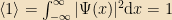
The wave function seems, in some way, to describe the “probability” that the particle will be found at (x, t).
The wave function itself, however, is not the probability; otherwise a single particle flying through no screens would show a sinusoidal distribution of positions, which it (evidently) doesn’t.

Schrödinger (and many others) puzzled over these properties a great deal. One key idea was about how to deal with (6). The simplest approach was to imagine that Ψ was a complex number, and the probability was given by some function of the magnitude of Ψ — say, $|\Psi|^2$ . One could also imagine adding more internal structure to Ψ, such as having it be vector-valued. It turned out that the simplest approach worked well; having Ψ be the square root of a probability, a.k.a. a probability amplitude, indeed matched all experiments.⁶ (And we will end up adding a great many internal degrees of freedom to Ψ as we go along in QM; for now, though, the simplest wave functions are just complex functions of position)

The most interesting idea, though, was for the simultaneous handling of (3) and (4).⁷ We know that Ψ is going to be subject to some kind of linear differential equation, by (2). Linear differential equations can be written in the language of linear algebra; after all, the set of functions forms a vector space, and if D is some arbitrary combination of x’s and $\partial$ ‘s, then $D(a\Psi_1 + b \Psi_2) = a D\Psi_1 + b D\Psi_2$ , so such a D is a linear operator. Its eigenvectors (commonly referred to as eigenfunctions, in this case) must form a basis for the set of all functions, and so on.

Now, if we look at the waveform in (3), there seems to be an obvious set of linear operators which would correspond to those very values of energy and momentum:

$P = -i\hbar\frac{\partial}{\partial x}$

$H = +i\hbar\frac{\partial}{\partial t}$

(We use H for the operator corresponding to total energy, H being short for the Hamiltonian operator which defines the total energy in classical mechanics; we will use lowercase p for the numeric [scalar] value of momentum, but a capital E for the scalar value of energy. This will be our one exception to the rule of using capital letters for operators, and the analogous lowercase letter to describe their eigenvalues) If we act with these operators on Ψ, we see

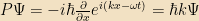
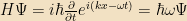
$P\Psi = -i\hbar\frac{\partial}{\partial x}e^{i(k x - \omega t)} = \hbar k \Psi$

$H\Psi = i\hbar\frac{\partial}{\partial t} e^{i(k x - \omega t)} = \hbar\omega \Psi$

If we are treating $|\Psi|^2$ as a probability weight, we should be able to talk about the mean value of physical quantities by taking the expectation value; but using these equations as a guide, we write out this general relationship in the slightly more cautious form

$\left<A\right> = \int {\rm d} x \Psi^\star(x) A \Psi(x)$ ,

where A is any one of these linear operators – X, P, H, and so on. Thus, for example, for a free wave

$\left<P\right> = \int {\rm d} x e^{-ipx/\hbar} (-i\hbar \partial_x) e^{ipx/\hbar} = p \left<1\right> = p$ .

Note that we must also, therefore, require that Ψ be normalizable —

$\left<1\right> = \int_{-\infty}^\infty|\Psi(x)|^2{\rm d}x=1$ .

This actually seems to rule out the free wave solution from being a valid wave function. In practice, on those occasions where we do have to deal with it — and it will show up, when studying free particles — we deal with it by letting space have some finite extent L, multiplying Ψ by an appropriate normalization factor, and at the very end taking L to infinity.

Given this relationship between waves, operators, and physically observable quantities, the main question which remains to be answered is what the wave equation actually is. Well, we know a natural relationship between energy and momentum; so did Schrödinger, and so armed with these ideas he immediately wrote down the famous Klein-Gordon Equation:

$(H^2 - P^2 c^2) \Psi = -\hbar^2\left(\partial_t^2 - c^2 \nabla^2\right)\Psi = m^2 c^4 \Psi$

…. oh.

You were expecting the Schrödinger equation?

Well, so was he. The problem was that Schrödinger wanted to write down a nice, relativistic equation. Unfortunately, the above equation has serious problems, which basically boil down to the fact that it’s second-order in time derivatives. This means that solutions come out in pairs with energies that are equal and of opposite sign — so you end up with a hierarchy of solutions of arbitrarily negative energy, and you can’t define decent physics at all. Schrödinger came up with this equation in 1921, and spent three years bashing his head against it until he heard that Heisenberg was getting close to publishing. Spurred into sudden action, he ditched any attempt at relativistic nicety, and instead published a paper based on the nonrelativistic equation that now bears his name:

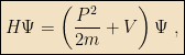
$\boxed{H \Psi = \left(\frac{P^2}{2m}+V\right) \Psi\ ,}$

or in terms of functions and derivatives,

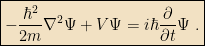
$\boxed{-\frac{\hbar^2}{2m}\nabla^2\Psi+V\Psi=i\hbar \frac{\partial}{\partial t}\Psi\ .}$

The first equation is written in terms of abstract operators, and is just the energy-momentum relationship of classical mechanics with an arbitrary potential energy, V. The second is rewritten in terms of derivatives of functions, and is the familiar form of the Schrödinger equation.

We’re going to spend much of the rest of this course looking at solutions of this equation for various potentials, and learning about the laws of physics from them. It will turn out that pretty much everything in nonrelativistic quantum mechanics comes down to understanding this one equation and the things one can measure it. But first, we’re going to plunge a bit further into understanding the equation “in its own right” — looking at it a bit more in the language of linear algebra, and finding some remarkable conclusions.

Next time: The Uncertainty Principle!

¹ I wish I could go into it here, but the calculation requires basic stat mech, which is beyond the scope of this class. However, you can find it in any intro to statistical mechanics; e.g., Kittel & Kroemer, Thermal Physics, chapter 4.

² This was one of Einstein’s three major papers of 1905; the other two were his paper on Brownian Motion, which was the final smoking-gun proof of the existence of atoms, and the special theory of relativity.

“It’s people like this who make you realize how little you’ve accomplished. It is a sobering thought, for example, that when Mozart was my age, he had been dead for three years.” — Tom Lehrer

³ The history of this, and the details of the experiment, are fascinating. If you’re interested, I suggest reading the first few chapters of Richard Rhodes’ The Making of the Atomic Bomb; they give a wonderful overview of the development of atomic and nuclear physics in the first half of the 20th century, and are remarkably readable.

⁴ If you read an older QM textbook such as Pauling & Wilson, you’ll see the text divided into discussing the “old quantum theory” and the “new quantum theory.” This “old” theory was basically the mass of pre-Schrödinger work; it’s somewhat fascinating to see how far people got by doing things as hard-to-justify as Bohr’s angular momentum rule. If you look at the very end of P&W, you’ll find a description of this radical new “matrix mechanics” of Dirac’s; it was very complicated for them to explain, because by and large physicists had never heard of matrices or linear algebra at the time; they were considered an obscure tool of mathematicians. It was only after Dirac’s major cleanup of QM using them in 1934, for which he basically derived the entire theory of linear algebra from scratch, that some mathematicians came by and said “Hey, you know that there’s a whole branch of math for this…” One other side effect of this is that, if you look at older texts and especially original papers, the derivations are a lot more complicated than the ones here.

⁵ And his theory was regarded as nearly insane. He proposed this in his Ph.D. thesis, and his degree was nearly not granted; it was only the personal intercession of Einstein, who thought the idea might have some merit, with his committee which saved him.

⁶ You may ask what justifies the formula $P = |\Psi|^2$ , as opposed to, say, $|\Psi|^4$ or something. The short answer is “because it matches experiment;” we’ll also see in the next lecture that it is particularly clean mathematically. But there has been research on this subject; oddly enough, it turns out that if $P \sim |\Psi|^n$ for n not an even integer, one could construct a “postselection machine” which could not only solve NP-complete problems in constant time, but also allow you to travel back in time with a special (and consistent) way of dealing with the grandfather paradox. (The first paper actually proves only poly time; the second paper improves it to a constant, as a side effect of being able to build time machines) So if you do manage to detect any deviation from the $|\Psi|^2$ behavior of probabilities, by all means, patent it! I suggest U. S. Patent No. 1.

⁷ What I’m about to give is a considerably simpler explanation than what Schrödinger originally did, in no small part because I’m going to use what we know about linear algebra quite freely. Schrödinger’s original approach started from Poisson brackets, and was quite rigorous, but as a result was also extremely complicated to explain; there’s a reason that QM was considered an advanced graduate subject for quite some time afterwards. I will shamelessly take advantage of nearly a century of improved mathematical techniques to give this the easy way.

Published in:

Quantum Mechanics

on August 4, 2010 at 10:10 Comments (6)
Tags: quantum mechanics

RSS feed for comments on this post.

6 Comments

On August 4, 2010 at 11:10 Russell said:

Hey Yonni – I’m really enjoying following your course!

(It has the added benefit that reading your posts makes me feel like I’m at least doing something productive while I avoid actual work.)

If only my insane ideas happened to match those of de Broglie… sigh.
- On August 4, 2010 at 11:11 zunger said:
  
  It’s a virtuous cycle; writing them makes me feel like I’m doing something productive while I avoid actual work.
On August 5, 2010 at 05:32 Rich said:

Add me to the list of those enjoying these posts.

It will turn out that pretty much everything in nonrelativistic quantum mechanics comes down to understanding this one equation and the things one can measure it.

Undergrad level QM became much easier for me when I realized the entire course (well, all the problems given anyway) was about boundary conditions. Unfortunately, this realization came after I took it.

Also, there’s an interesting discussion going on at Chad Orzel’s blog about teaching Stat. Mech. that matches well with my experience.
On August 5, 2010 at 10:54 moof said:

tiny nit: it’s Niels Bohr, not Neils.

Some more background of what a “free wave” is would have been nice.
- On August 5, 2010 at 11:12 zunger said:
  
  Whoops — typo. Fixed.
  
  A free wave is a solution to the wave equation in the absence of any background forces or potentials; it’s the equation which describes a wave propagating in a medium without any forces on it. It’s the same equation for, e.g., sound waves, light waves, and so on, and its solution (in an infinite, empty space, so that there aren’t any complicated boundary conditions) is $e^{i(kx-\omega t)}$ . That’s a sine wave with wave number k, with the wave peaks moving along at a velocity $\omega/k$ .
  
  All of the usual rules of optics and so on follow from this; e.g., you can get the formula for the interference pattern you see when you push light through slits, gratings, and so on by adding up a bunch of free waves of the relevant sort. (For light, the wave velocity is just the speed of light)
  
  Does that answer your question?
  - On August 5, 2010 at 17:53 moof said:
    
    Ah, yes indeed, that answers it. I wasn’t sure if the term was referring to something specifically in QM, for a particular medium, etc. (There are plenty of equations in QM that look simple and innocuous, after all.)
    
    I’d also note that this is the first time I’d seen “capital letters, as a rule, are operators” called out explicitly. Everything else I’ve seen seemed to assume you’d pick it up eventually – which I guess is true, but it’s quite nice to see the context made explicit.

Comments are closed.

Yonatan Zunger’s Blog

From Machine Learning to the Middle East