Yonatan Zunger’s Blog

Alright, enough with the mathematical abstraction! This post, and the next quite a few posts, will all be looking at very concrete, physical examples, applying the methods of quantum mechanics and seeing what we can see. Today, we’re going to start with the simplest possible system that has nontrivial dynamics: a system with only two states in it. In a sign of great creativity, this is normally referred to as “the two-state system.”

Since the time evolution of a single eigenstate of the Hamiltonian is just a phase rotation, which (as we saw last time) means that expectation values never change, the simplest Hamiltonian we could possibly imagine which still has any dynamics at all would be one which acts on a two-dimensional vector space of states. Note that this isn’t the same as a particle in a two-dimensional space; having even one dimension of space implies an infinite-dimensional space of functions on that space. No, if we want to have a genuinely two-state system, we need to have one without any momentum or derivatives at all.

Does nature provide any situations like this? Well, for there to be no motion or momentum in the system, the particle(s) under study need to be effectively nailed down. This isn’t difficult; if we are studying (say) atoms in a solid, then so long as the energies we’re dealing with are considerably less than those required to make the atom move within the solid, then to a good approximation the position is a constant and there will be no momentum term in the Hamiltonian. (Or equivalently, if the particles are very massive, so that our potential V) And nature has also provided us with an excellent example of a two-state system, in the form of spin.

Spin is a property which we will discuss at great length later on; it turns out to physically represent an “intrinsic angular momentum” which some particles have. For today’s purposes, all we need to know is that some particles have such a property, and the internal state of those particles is described by a two-dimensional vector.¹ This vector is acted upon by the three spin operators:

.

The “vector” of these three operators acts like angular momentum; in particular, if a charged particle with spin is placed in a magnetic field, it experiences a potential

.

Here e is the charge of the particle; m is its mass; is the vector of spin operators; is the applied magnetic field; and g is a dimensionless constant characteristic of the particle called the gyromagnetic ratio. These ratios have been measured for a wide range of materials; one of the great triumphs of quantum field theory is the calculation of the gyromagnetic ratio of the electron to 14 decimal places from first principles, giving an insanely precise value — which matches experiment! — of .

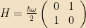
So let’s experiment with a Hamiltonian which consists of nothing but this potential, acting on a spin-1/2 particle which has been nailed down firmly to the lab bench. First, say we apply a magnetic field in the z-direction:

.

This Hamiltonian is already diagonal, so it’s trivial to know the eigenvectors and their eigenvalues; they are simply 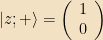and , with eigenvalues ; here I’ve defined

.

The eigenvectors were labelled with a letter z to indicate that these are the eigenvectors for fields in the z-direction (and thus are eigenvectors of ), and with ± to indicate the directions in which they point. If on the other hand, the magnetic field had been pointing in the x-direction, we would have had

.

We can find the eigenvalues by directly solving the eigenvalue equation for this matrix — . The corresponding eigenvectors satisfy

;

if we add the normalization condition on the eigenvectors as well, we find

.

Note that the energies are the same as in the z-case, which makes sense by symmetry; our definition of which axis is which is wholly arbitrary.

Exercise: Find the corresponding eigenvectors and eigenvalues for a field in the y-direction.

Now let’s do something more interesting. Imagine that the system started out in the state , but we applied a magnetic field in the z-direction. How would it evolve over time? The eigenvectors of the Hamiltonian are , so we first write the initial state of the system in terms of those:

.

Then using our time-evolution formula from last time, it follows that

.

To see what this means, let’s measure some physical quantities:

.

Thus a magnetic field in the z-direction causes the spin to rotate in the xy-plane with angular frequency . But this is exactly what would happen to a classical particle with the same magnetic moment; so classical physics intuition still makes sense!

There actually isn’t that much more that we can do with just this Hamiltonian. For any constant B-field, we can find the eigenvectors, write any initial state in terms of them, and see how it evolves. In every case, magnetic fields will cause the component of the magnetic moment perpendicular to the field to rotate about the field axis, just like in classical physics. So to make something more interesting happen, next time we’ll turn on a time-varying field and see what it does.

Next Time: Nuclear magnetic resonance

¹ More specifically: particles have a “total spin” s which is an integer or a half-integer; they have 2s+1 internal states. They are always acted upon by three operators , and the commutation relationship between those operators is always the same, but the expression as matrices depends on the spin. Electrons, protons, neutrons, and about half of all nuclei have spin 1/2; other nuclei have spins ranging from zero to six.