Nuclear Magnetic Resonance

Last time, we looked at a particle with spin 1/2 in a constant magnetic field. We saw that, like with a classical magnetic dipole, this field caused the magnetic moment to rotate around the field axis. Whenever we encounter a rotating body, a natural thing to try to do is to apply a rotating force to it and see if we can make it resonate.¹ Today we’ll do that and see what happens.

To create a resonance, we’re going to simultaneously apply two magnetic fields: one big field of strength B in the z-direction, and a second field of strength b oscillating in the xy-plane. Our Hamiltonian is once again $H=(eg/2m) \vec{S}\cdot\vec{B}$ , or

$\begin{array}{rcl} H &=& \frac{eg\hbar}{4m}\left(\begin{array}{cc} B & b e^{-i\Omega t} \\ b e^{i\Omega t} & B \end{array}\right) \\ &=& \frac{\hbar\omega}{2}\left(\begin{array}{cc}1&\gamma e^{-i\Omega t}\\ \gamma e^{i\Omega t}&-1\end{array}\right)\ , \end{array}$

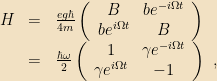
where as before we have defined

$\omega\equiv\frac{egB}{2m}$

as well as

$\gamma\equiv\frac{b}{B}$ .

To make this example physically concrete, say we were to start out with the spin originally in the $\left|z;-\right>$ state. (This is the ground state of the system whenever the oscillating field is turned off, so it’s a natural place to start) If we apply the oscillating field, what is the probability that the particle will end up in the $\left|z;+\right>$ state?

Since the Hamiltonian is explicitly time-dependent, the Schrödinger equation isn’t a simple eigenvalue equation. Instead we get a pair of coupled differential equations for the two components of $\left|\Psi\right>$ , $c_+$ and $c_-$ .

$\frac{\hbar\omega}{2}\left(\begin{array}{cc}1&\gamma e^{-i\Omega t}\\\gamma e^{i\Omega t}&-1\end{array}\right)\left(\begin{array}{c}c_+\\c_-\end{array}\right) = i\hbar\left(\begin{array}{c}\dot{c}_+\\\dot{c}_-\end{array}\right)$

$\dot{c}_+ = -\frac{i\omega}{2} c_+ - \frac{i\omega\gamma}{2}e^{-i\Omega t} c_-$

$\dot{c}_- = +\frac{i\omega}{2} c_- - \frac{i\omega\gamma}{2}e^{i\Omega t} c_+$

We can solve these by decoupling the equations. First, from the first equation it follows that

$c_- = \frac{2i}{\omega\gamma} e^{i\Omega t} \left(\dot{c}_+ + \frac{i\omega}{2}c_+\right)$

and then from the second we get

$\gamma\dot{c}_- = -\frac{i\omega}{2}e^{i\Omega t}\left(\gamma^2+1\right) c_+ - e^{i\Omega t} \dot{c}_+$ .

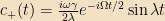
Then taking the derivative of the $c_+$ equation, we see

$\begin{array}{rcl} \ddot{c}_+ &=& -\frac{i\omega}{2}\dot{c}_+ + i\Omega\left(\frac{i\omega\gamma}{2}\right)e^{-i\Omega t}c_- -\frac{i\omega\gamma}{2}e^{-i\Omega t}\dot{c}_-\\&=&-\frac{i\omega}{2}\dot{c}_+-i\Omega\left(\dot{c}_++\frac{i\omega}{2}c_+\right)-\frac{i\omega}{2}\left(-\frac{i\omega}{2}\right)(\gamma^2+1)c_++\frac{i\omega}{2}\dot{c}_+\\&=&-i\Omega\dot{c}_++ \frac{\omega}{2}\left[\Omega-\frac{\omega}{2}(\gamma^2+1)\right]c_+\end{array}$ .

This is just a second-order equation with constant coefficients, so we can immediately solve it by writing $c_+=e^{i\chi t}$ ; substituting this in gives the simple algebraic equation

$\chi^2 +\chi\Omega +\frac{\omega}{2}\left[\Omega-\frac{\omega}{2}(\gamma^2+1)\right] = 0$ .

The solutions to this equation are

$\chi=-\frac{\Omega}{2}\pm\frac{1}{2}\sqrt{(\Omega-\omega)^2+\omega^2\gamma^2}\equiv-\frac{\Omega}{2}\pm\lambda$ .

Therefore

$c_+(t) = e^{-i\Omega t/2}\left[ A e^{i\lambda t} + B e^{-i\lambda t}\right]$ .

Our initial condition was that the particle started out in the $\left|z;-\right>$ state, i.e. $c_+(0)=0$ and $c_-(0)=1$ . Using our expression for $c_-$ above, the latter translates into $\dot{c}_+(0) = -\frac{i\omega\gamma}{2}$ . So

$c_+(0) = A+B = 0$ , and

$\dot{c}_+(0) = -\frac{i\Omega}{2}c_+(0)+i\lambda (A-B) = -\frac{i\omega\gamma}{2}$ ,

and so $A=-B=\omega\gamma/4\lambda$ , or

$c_+(t) = \frac{i\omega\gamma}{2\lambda} e^{-i\Omega t/2} \sin\lambda t$ .

As a sanity check, we can evaluate $c_-$ using our earlier formula;

$\begin{array}{rcl}c_-(t)&=&-\frac{2i}{\omega\gamma}e^{i\Omega t}\frac{i\omega\gamma}{2\lambda}\left[-\frac{i\Omega}{2}e^{-i\Omega t/2}S+e^{-i\Omega t/2}\lambda C+\frac{i\omega}{2}e^{-i\Omega t/2}S\right]\\&=&-\frac{1}{\lambda}e^{i\Omega t/2}\left[\frac{i}{2}(\omega-\Omega)\sin\lambda t+\lambda\cos\lambda t\right]\end{array}$ ,

(writing S for $\sin\lambda t$ etc.) and verify that

$\begin{array}{rcl}|c_+|^2+|c_-|^2&=&\frac{\omega^2\gamma^2}{4\lambda^2}S^2+\frac{1}{\lambda^2}\left[\lambda^2C^2+\frac{1}{4}(\Omega-\omega)^2S^2\right]\\&=&\frac{1}{\lambda^2}\left[\left(\frac{\omega^2\gamma^2}{4}+\frac{1}{4}(\Omega-\omega)^2\right)S^2+\lambda^2C^2\right]\\&=&\frac{1}{\lambda^2}\left[\lambda^2S^2+\lambda^2C^2\right]=1\ ,\end{array}$

and so probability is conserved.²

The probability of ending up in the + state is simply

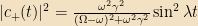
$|c_+(t)|^2=\frac{\omega^2\gamma^2}{(\Omega-\omega)^2+\omega^2\gamma^2}\sin^2\lambda t$ .

This is known as Rabi’s Formula.³ The interesting feature of this equation is the coefficient of the sine. The amplitude of oscillations gets small whenever $|\Omega-\omega|$ gets big, and goes to one whenever $\Omega=\omega$ . In fact, this coefficient has the structure of a classical resonance peak; whenever the driving frequency is close to the resonant frequency of the system, oscillations get large, even if the driving force ( $\gamma$ ) is small. The smaller $\gamma$ is, the narrower the peak becomes.

Using this result

There are two common ways to measure this peak in the lab. The simplest one is to note that the total energy of the system oscillates with the same phase and frequency as $|c_+|^2$ . There are two ways to see this; directly, by calculating $\left<H\right>$ [Exercise: Do it!] and more simply by noting that in the limit $\gamma\ll 1$ , the eigenstates are approximately the original $\left|z;\pm\right>$ eigenstates, and whenever we make a transition between the two states we must therefore be paying the energy difference $\hbar\omega$ . Conservation of energy still holds; if the total energy of this particle is changing, it’s because (since we have a time-varying potential) some external system is injecting energy into the system. That time-varying potential is simply the oscillating magnetic field, and one can observe the oscillation very simply by attaching an oscilloscope to the leads powering the oscillating field.

With this sort of instrument — one powerful magnet producing B, one oscillating magnet with its power drain being monitored — one can then adjust Ω until the power drain is at maximum. This gives a measurement of ω, and therefore (since B is known) of the ratio $eg/m$ , which is a characteristic of the material being studied. One can then go ahead and tabulate these values for a wide range of materials, and use this to identify substances.

Note that in practice, the material at the center of the experiment will not be a single, spin-1/2 particle; it will be a macroscopic agglomeration of stuff, including electrons, protons, nuclei, and so on. The experiment can nonetheless work; each spin-1/2 particle will be resonating independently, and by scanning over different values of Ω one can encounter each respective resonance peak. In a good experimental situation, one peak should stand out; e.g., if one places a crystal of some fairly pure element in the center, the amount of that will greatly exceed the amount of air (etc) in the system. Furthermore, peaks due to electrons and peaks due to nuclei will be well-differentiated; they have similar values of e and g, but their masses differ by several orders of magnitude. In practice, the effective gyromagnetic ratio of electrons depends a great deal on their molecular state, and the large number of electrons in different states makes the signal less clean; so for identifying elements, the most useful peaks to study are the nuclear peaks. This technique is called nuclear magnetic resonance.

The second way to measure the Rabi peak is due to Lauterbur and Mansfield, who realized that by using multiple magnets, they could effectively “aim” the oscillating field at a fairly precise point in 3-dimensional space. Rather than using this to identify unknown substances, they used it to measure the density of a known substance, specifically Hydrogen. In this configuration, directly measuring the resonant load on the magnets isn’t the most precise method; instead, the oscillating field is run for a short burst, half of a resonant cycle time; this excites the Hydrogen nuclei into the + state, (relative to the large B-field produced by a single big magnet) and when the oscillating field is deactivated the nuclei drop back into the – state, emitting the energy difference in the form of photons. For the sizes of B-field used in practical devices (generally between 1 and 2 Tesla, which means that one can easily achieve a γ of $10^{-3}$ without running in to interference from ambient magnetic fields) these photons are in the radio-frequency range, and so are easy to detect; their overall intensity reveals the density of Hydrogen nuclei in the region being probed.

What’s especially useful about this is that, by rastering the point over space, one can build up a map of the three-dimensional density of Hydrogen (and thus, to a good approximation, of organic matter, which tends to have all its free bonds filled in with Hydrogen) over a volume without having to either dissect it or fill it with radioactive tracer elements. (Which was the previous best way of getting 3D images of things) This can be handy if the volume contains something like a person, who might otherwise object to being dissected or filled with radioactive tracers. This technique, magnetic resonance imaging, led to major advances in medicine, and Lauterbur and Mansfield shared the 2003 Nobel Prize for their work.

¹ In the same vein that a natural thing to try to do when you see a big red button is to poke it. Physicists are easily amused.

² It’s always good to run some sanity checks after doing any heavy algebra.

³ For which he won the 1944 Nobel in Physics. See what you could have done had you just learned quantum mechanics a bit earlier?

Published in:

Quantum Mechanics

on August 24, 2010 at 10:00 Comments (1)
Tags: quantum mechanics

RSS feed for comments on this post.

One Comment

On September 6, 2011 at 11:39 Nuclear Magnetic Resonance: Volume 38 (Specialist Periodical Reports) | Medical Imaging Science said:

[…] jQuery(function() { // jQuery('#amzngalleryloading').hide('slow'); jQuery('a.amznfancybox').fancybox({ 'transitionIn' : 'elastic', 'transitionOut' : 'elastic', 'speedIn' : 600, 'speedOut' : 200, 'overlayShow' : false }); jQuery('#amzngallery').show('slow'); }); #split {}#single {}#splitalign {margin-left: auto; margin-right: auto;}#singlealign {margin-left: auto; margin-right: auto;}.linkboxtext {line-height: 1.4em;}.linkboxcontainer {padding: 7px 7px 7px 7px;background-color:#eeeeee;border-color:#000000;border-width:0px; border-style:solid;}.linkboxdisplay {padding: 7px 7px 7px 7px;}.linkboxdisplay td {text-align: center;}.linkboxdisplay a:link {text-decoration: none;}.linkboxdisplay a:hover {text-decoration: underline;} function opensingledropdown() { document.getElementById('singletablelinks').style.display = ''; document.getElementById('singlemouse').style.display = 'none'; } function closesingledropdown() { document.getElementById('singletablelinks').style.display = 'none'; document.getElementById('singlemouse').style.display = ''; } Have a look:Spin Dynamics: Basics of Nuclear Magnetic Resonance OffersNuclear Magnetic Resonance […]

Comments are closed.

Yonatan Zunger’s Blog

From Machine Learning to the Middle East